Do you have some data and a model that you want to fit? Well here's the website for you (see caveats)!
On this website you can input a model function defined by a set of parameters, including those that you want fit, as well as your data, and it will run a statistical sampling algorithm to estimate the posterior probability distributions of those parameters.
This site makes use of the Bayesian inference Python package Bilby to access a selection of statistical samplers.
Beyond Markov chain Monte Carlo (MCMC), users are able to select from a variety of statistical samplers and it is encouraged to trial a variety to achieve the best performance for your model.
EXAMPLES
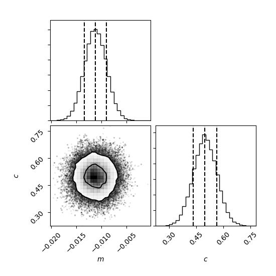
This site generates two plots: one of the marginalised posterior plots for each parameter that the user defines...
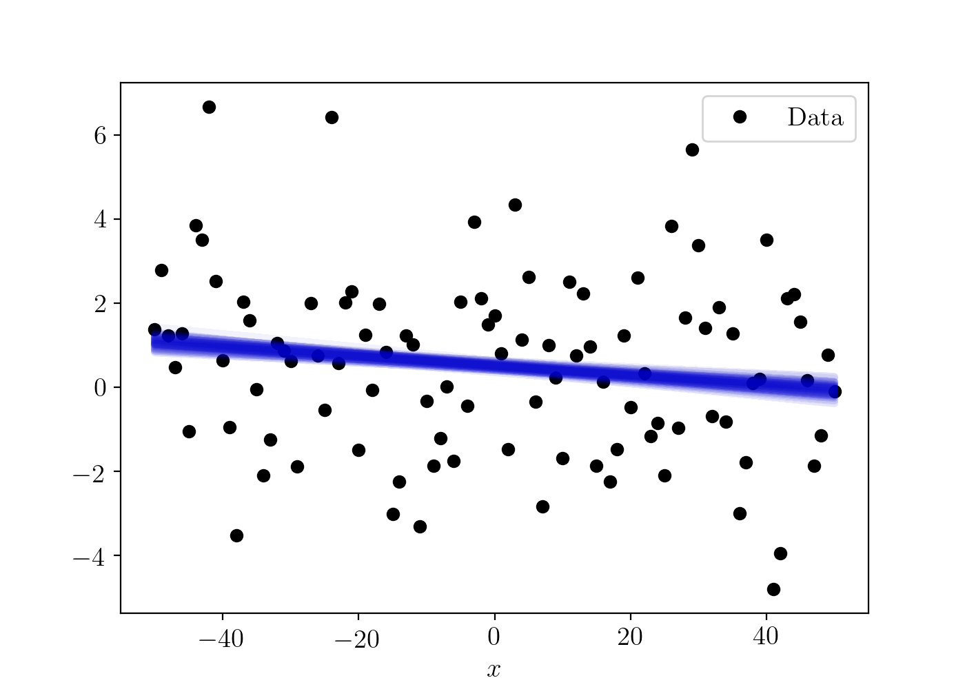
... and another showing the distribution of all the best fit models that were drawn randomly from the posterior distribution.
While full instructions and explanations can be found here, the following video showing how to use the website might also be useful. In this case a basic linear model and a small data set were used for simplicity.
INPUT
Instructions for using this page can be found below the input options.
NOTE - Functions within piecewise must be written as lambda functions.
For example, if all values of x greater than five are multiplied by 'a', and all less than or equal multuplied by 3, it would appear as piecewise(x,[x<=5,x>5],[lambda x:x^3, lambda x:x^a])
More information on how to use and input a piecewise equation can be found here.
Any results will be available for 15 days following completion. They will then be deleted, so please download any results that you would like to keep for longer.
Firstly, you must input the model that you want to fit to your data. When inputting this model you can use the standard operators "+", "-", "*" (multiplication), "/" (division). Allowable functions (such as trigonometric functions) and constants are listed below. To raise a value to a given power use either "^" or "**".
It is advised to plot just your data points initially to give an indication of what model you could use.
When entering the model be careful to use parentheses to group the required parts of the equation. Click here to show an example input model.
To input the model \(2.2 \sin{(2\pi f t)} + a t^2 - \frac{e^{2.3}}{b}\) you would write:
2.2*sin(2.0*pi*f*t) + a*t^2 - (exp(2.3)/b)
The webpage will parse this information and extract the parameters \(f\), \(t\), \(a\) and \(b\).
Parameter types
Once the model is submitted you can choose each parameter's type:
constant: the parameter is a fixed constant that you can define a numerical value for;
variable: the parameter is a variable that you would like to fit and for which you will need to define a prior (see here for information on the prior type);
independent variable / abscissa: the parameter is a value, or set of values, at which the model is defined (e.g. in the above example the t (time) value could be such a parameter) that you can input directly or through file upload (uploaded files can be plain ascii text with whitespace or comma separated values). Currently only one parameter can be given as an independent variable, i.e. only one-dimensional models are allowed.
Log(Uniform): this is a constant probability distribution in the logarithm of the parameter, defined within a minimum and maximum range, with zero probability outside that range. This is a non-informative prior for a scale parameter (i.e. a parameter that is invariant to scalings and can only take positive values);
Exponential: this is an Exponential probability distribution (\(e^{-x/\mu}\)) for which the mean, μ, must be specified. This is the least informative distribution if only the mean is known.
If you are unsure about what is best to use then a Uniform distribution with a range broad enough to cover your expectations of the parameter is the simplest option.
Data input
Input the data that you would like to fit the model to. You can directly choose to input values directly in the form below (with whitespace or comma separated values), or upload a file containing the data (again with whitespace, or comma separated values). The number of input data points must be the same as the number of values input for the independent variable/abscissa parameter provided above.
input a single known value for the standard deviation, σ, of noise in the data;
input a set of values (either directly into the form as a set of whitespace or comma separated values, or though uploading an ascii text file of the values) of the standard deviation of the noise, with one value per data point;
choose to include the noise standard deviation as another parameter to be fit (i.e. if it is unknown). If you choose this option then a prior (as above) is required.
Student's t: the Student's t likelihood is similar to the Gaussian likelihood, but it does not require a noise standard deviation to be given (the noise is assumed to be stationary over the dataset and has been analytically marginalised over).
Poisson: the Poisson distribution is similar to the Gaussian, however it deals with discrete random variables, such as counting a radioactive decay source. The data input therefore is required to be integer counts and only positive values.
Sampler Inputs
Through Bilby one can select from a variety of statistical samplers, each utilising a slightly different algorithm to sample from the posterior distribution of the parameter space. The samplers available are broken down into
two separate classes, Markov chain Monte Carlo methods (see emcee and PyMC3) and Nested Sampling algorithms (see Dynesty and Nestle).
emcee is an MCMC algorithm that aims to draw samples (a chain of points) from the posterior probability distributions of the parameters. You need to tell it how many points to draw. There are three inputs required:
No. of ensemble points ("walkers"): this is essentially the number of independent chains within the MCMC. This needs to be an even number and in general should be at least twice the number of fitting parameters that you have. Using a large value (e.g. 100) should be fine, but you could run into lack-of-memory issues if the number is too high (1000s);
No. of iterations: this is the number of points per chain for each of the ensemble points. The product of this number and the number of ensemble points will be the total number of samples that you have for the posterior;
No. of burn-in iterations: this is the number of iterations (for each "walker") that are thrown away from the start of the chain (the iteration points above come after the burn-in points). This allows time for the MCMC to converge on the bulk of the posterior and for points sampled away from that to not be included in the final results.
Tips
Fitting a multimodal distribution? Try increasing the number of walkers!
Does your data have little noise(SNR)? Try increasing the number of burn in iterations!
Dynesty provides an implementation of the Nested Sampling algorithm, with access to a variety of different sampling method (although here it is currently fixed to used a MultiNest-based sampling method). Nested sampling is similar to the MCMC method, however the nature of the sampling allows one to calculate the integral of the probability distribution, and as a by-product can produce samples from the marginal posterior distributions. For Dynesty, only one input is required:
No. of live points : this is described in greater detail here. This needs to be a positive integer and in general should be at least 1 greater than the number of fitting parameters that exist.
Nestle provides an implementation of the Nested Sampling algorithm, with access to a couple of different sampling method (although here it is currently fixed to used a MultiNest-based sampling method). Nested sampling is similar to the MCMC method, however the nature of the sampling allows one to calculate the integral of the probability distribution, and as a by-product can produce samples from the marginal posterior distributions. For Nestle, two inputs are required:
No. of live points : the number of active points, a positive interger at least one greater than the number of fitting parameters that exist.
Method : How the sampler chooses new points within the target parameter space. Currently can choose from 'Classic', 'Single' or 'Multi'. Further information can be found here
PyMC3 is another MCMC sampler, which can uses a variety of efficient sampling algorithms. The output is a chain of points drawn from the posterior probability distributions of the parameters. For PyMC3, three inputs are required:
No. of draws : The number of sample draws from the posterior per chain.
No. of chains : The number of independent MCMC chains to run.
No. of burn-in iterations: this is the number of iterations that are thrown away from the start of the chain (the iteration points above come after the burn-in points). This allows time for the MCMC to converge on the bulk of the posterior and for points sampled away from that to not be included in the final results.
If in doubt use the defaults and see how things turn out.
ALLOWABLE FUNCTIONS AND CONSTANTS
Here is a list of allowable functions within your model. When entering your model use the form given in the monospace font, with the function argument surrounded by brackets, e.g. sin(x).
The sampling algorithms provided are not guaranteed to produce sensible results every time, and your output may contain errors or look odd. Some information and trouble shooting for the samplers can be found here.
For very high SNR models, it is possible for MCMC solutions to converge very slowly as exploring the parameter space becomes difficult. For such cases, solutions will take longer to be produced.
If users really want to understand what is being done by this code I would advise learning about Bayesian analyses and Markov chain Monte Carlo methods. I would also advise learning Python, or another programming language, and coding the analysis up themselves, particularly if you have a more complex problem. However, this site aims to be useful starting point.